Google Sheets is a very useful application created by Google and it fulfills most of the needs of Microsoft Excel. In this post, I will guide you on How To Make A Table In Google Sheets And how you can make it beautiful and make the google sheets attractive.
To create a Google sheet you need a Google account which means a Gmail account. If you don't have a Gmail account then create one.
First, go to the Google search and type “Google Drive” after that click on the first result a window will open then click on go to the drive options and a new window will open click on the new options where you can find the Google sheet.
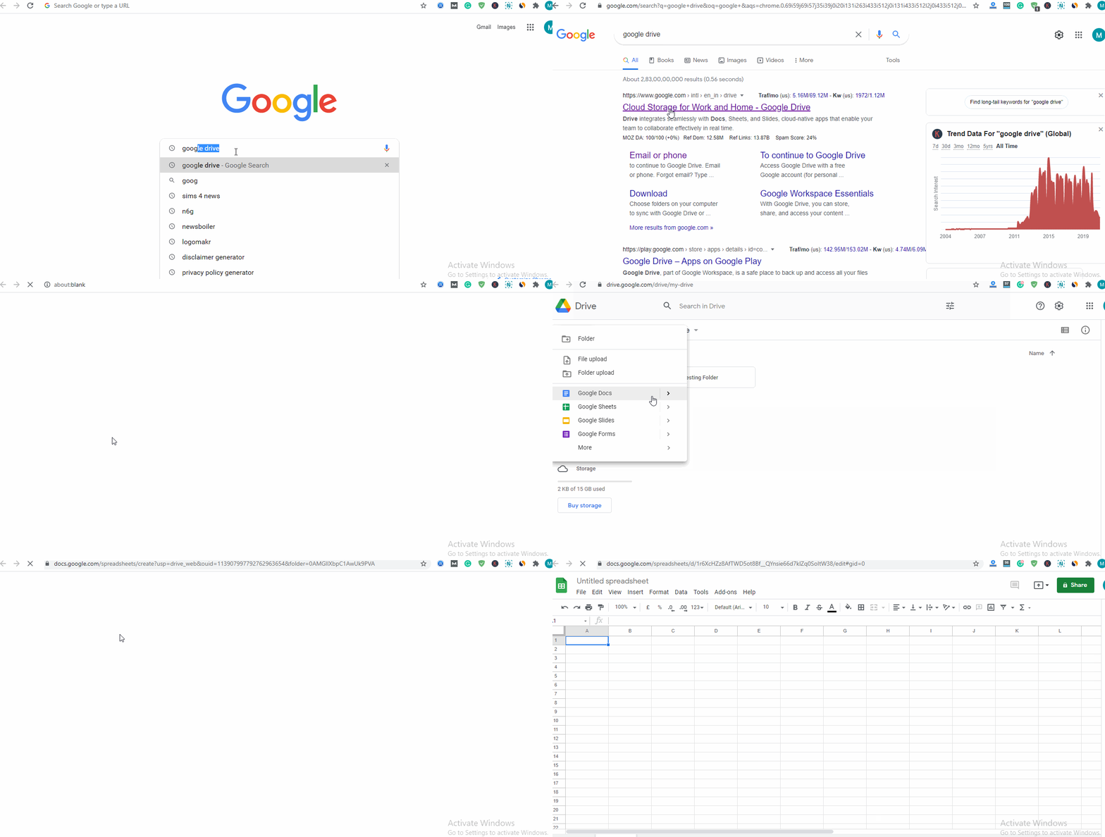
From the above image, you can understand How To open google drive to create a google sheet. Now move on to the next step
How To Make A Table In Google Sheets
Now you understand how to open a google sheet and the first step to create a google sheet. Now after open the google sheet you have to type some data for the table just like below and after that, we will move on to the next step
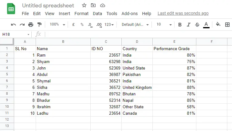
Now you created a table but the table is ugly so you have to give the proper format of the table. Now move on to how you can give the proper format so that the table looks great and attractive.
How To Format A Google Sheet
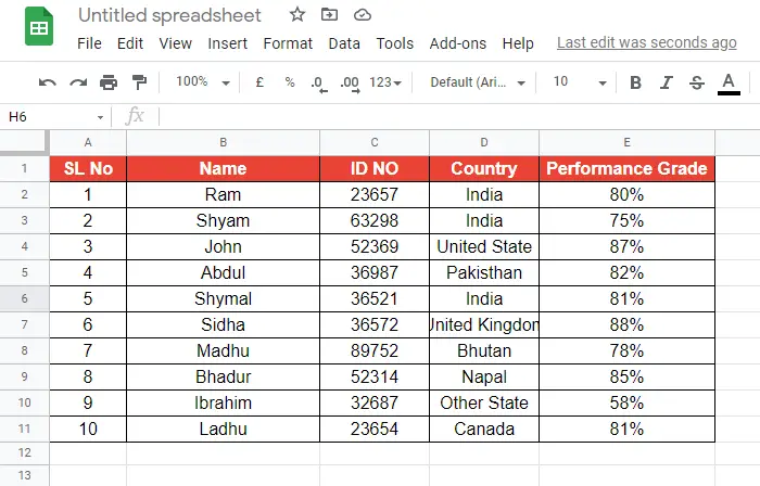
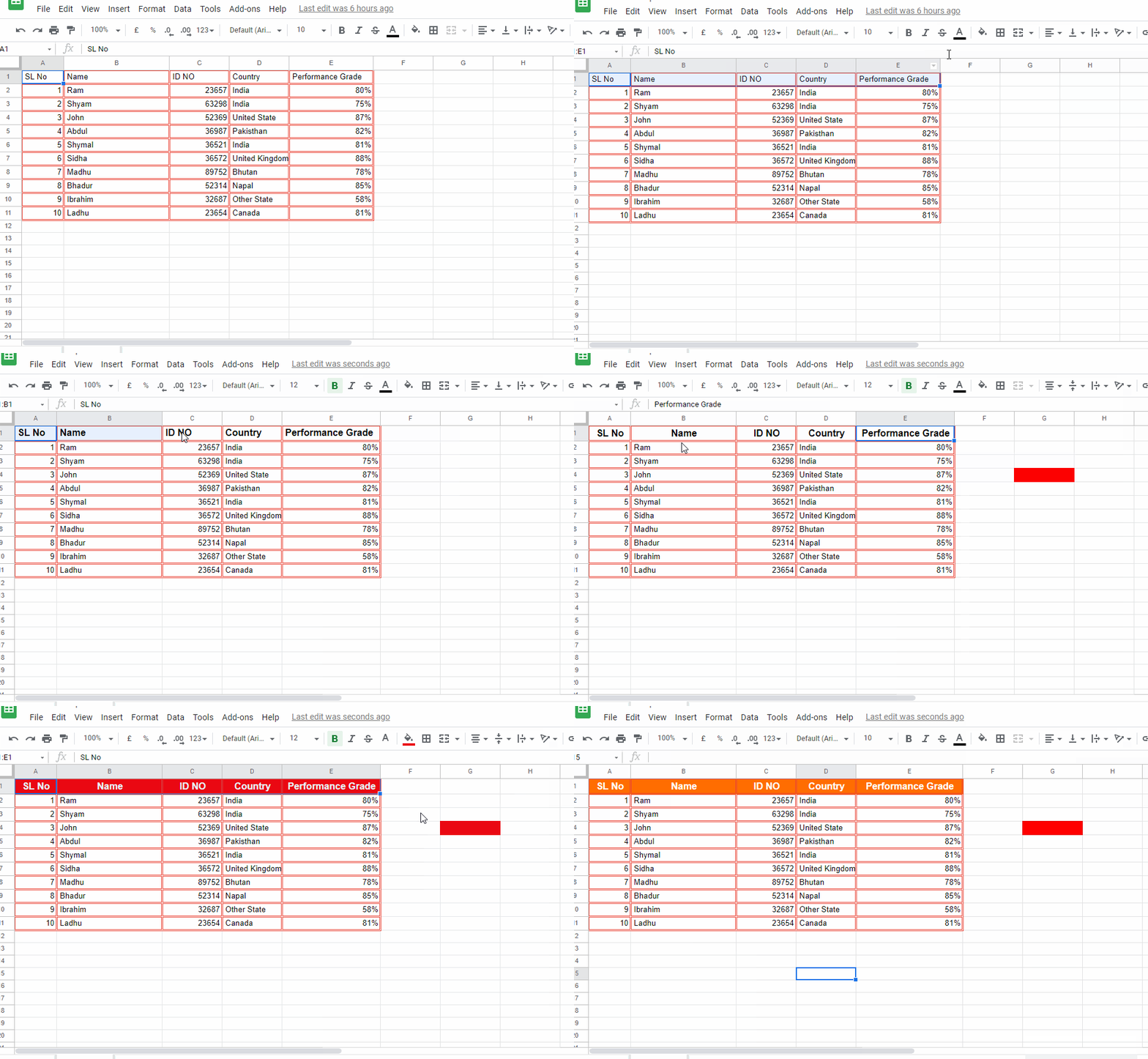
You can see the above table is not formatted that's why the table does not look attractive so you have to format Google sheets properly so that the table looks like the one below
How To Create a Border For The Table
You can see in the above picture that the Google sheet table border separates the row and column from each other. So how you can create a border for a table?
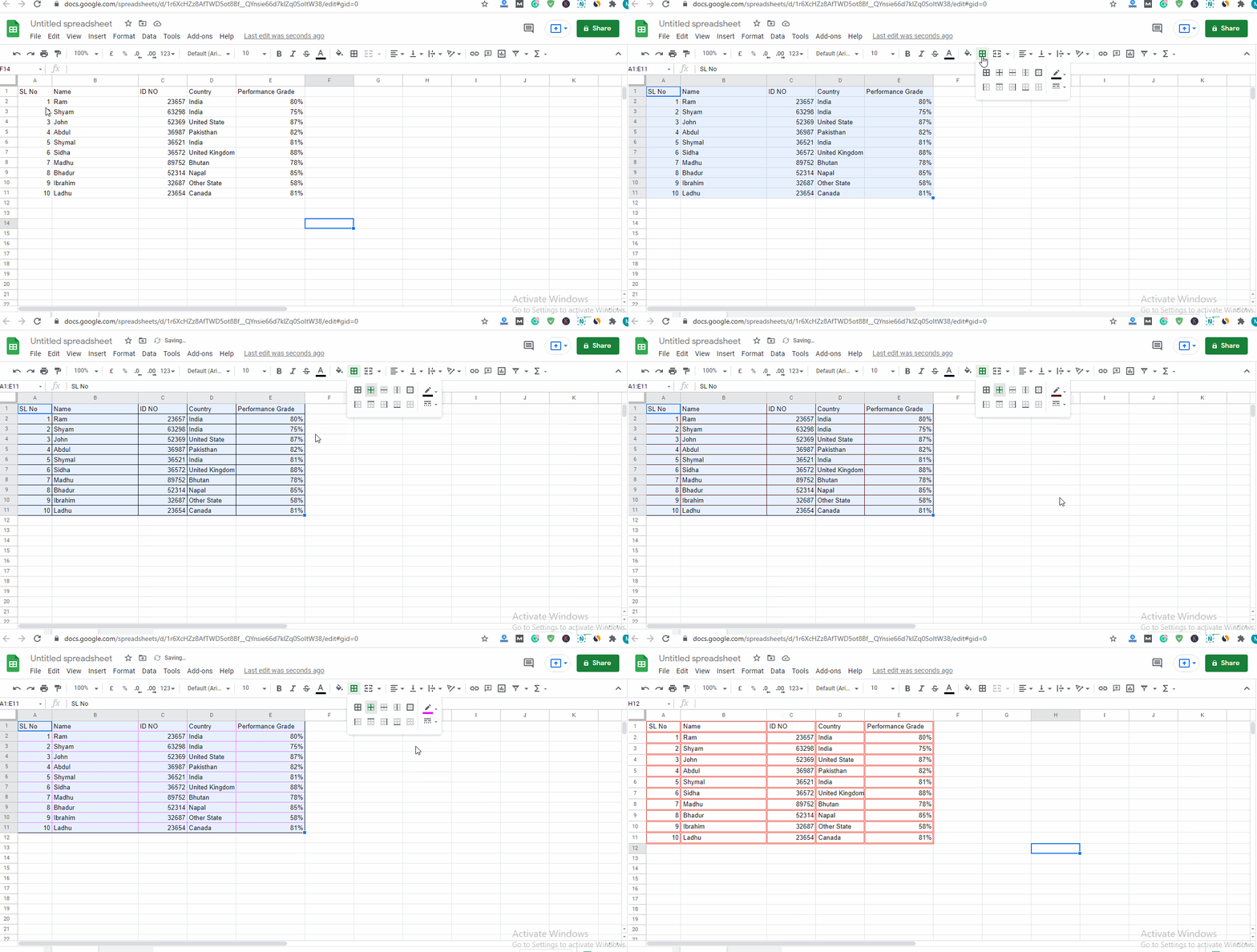
First, select all the fill areas of the table and then click on the borders options where you can create borders for many formats. Just see the below image to understand properly.
Format The Header
Now you understand that how to set the border to a Google sheet table. Now learn how you can format the header so that the header looks very attractive.
First, just select the header and after that click on the bold options to bold the header, if you want to set different background then click on the background options and select the color to change the color. You can also change the header color and for that click on the header color options and select the color according to your needs. Just check the image below to understand better.
How To Aligning Table Column
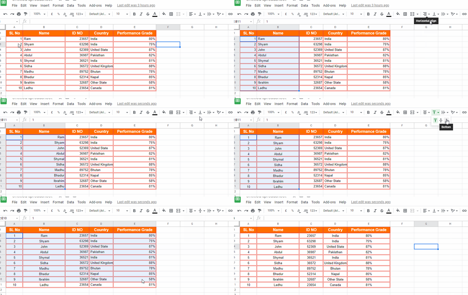
Now the next step is how you can align the table column. You can align the Google sheet column in three ways. No 1 way is to align the column left, the second way is to align the table column to the right and the last or third way is to align the table column to the center.
To align the table column left first select the whole table or the exact row you want to align then click on the alignment options where you can see three options the first one is left, the second is center and the third one is right. Click anyone according to your choice.
In the alignment options, you can find two types of alignment one is horizontally aligned and the second one is vertical-align. Choose the type of aligning options to align your table column.
You may also Like: How To Create WordPress Blog Free Step By Step
Format The Table Data
Now you have to format the data or number according to your need for example you can add a currency sign before the number, add the decimal value into your table data. Add the thousands separation for the big numbers and set the number according to decimal format.
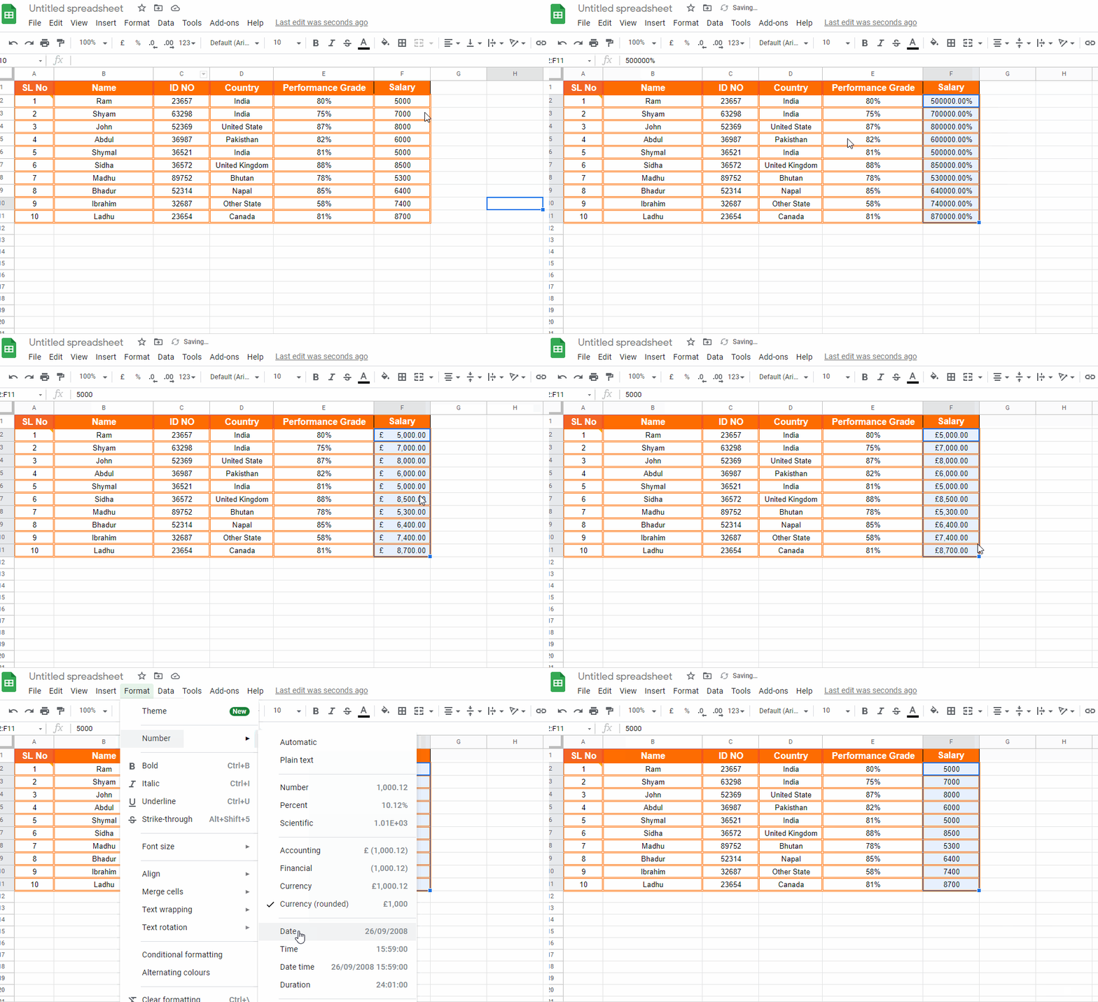
Here in the above image, you can see that you can set the number as a decimal number, like date, as time, add currency value, add a percentage, format the number according to accounting, rounded currency, as a financial number, as plain text, and more. Just set the number according to your needs.
How To Do Bold, Italic, Underline, Strike-through, And More
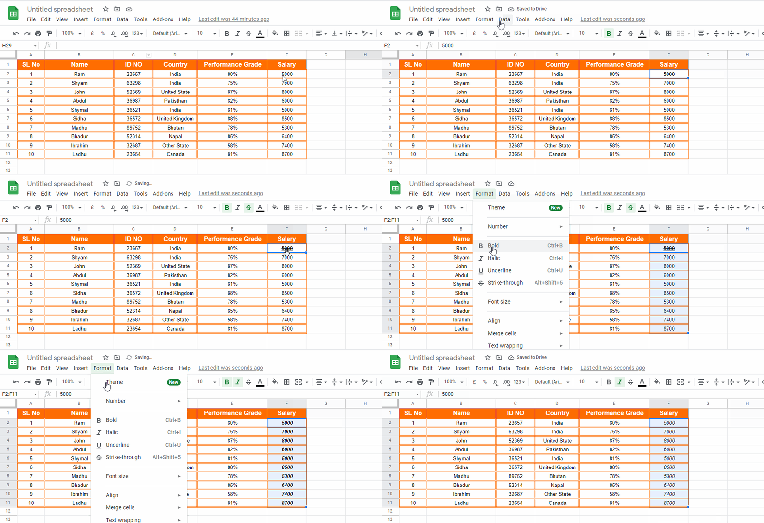
You can easily do bold, italic, or underline or strike-through a column or a row or a particular room of a column or a row. To do that first select the particular row or column or exact room after that click on the bold options if you want to do blood, or click on the italic to do italic, and click on the underline to underline the whole row or column text.
Just follow the image below to understand how to do blood, italic, or underlined or strike-through. Follow the image carefully
What About Text Wrapping
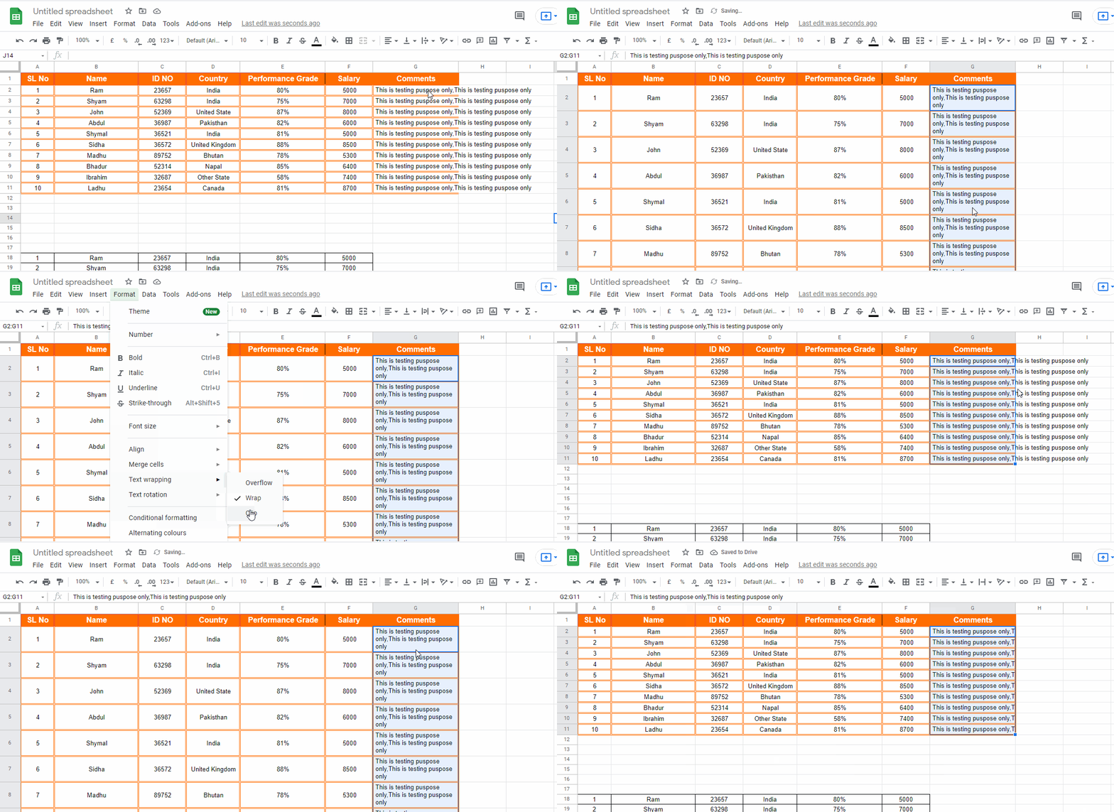
Text wrapping is a format where you can format your table text in three ways. The first way is overflow the second way is a wrap and the third one is the clip.
In the overflow options, your text will overflow on the box, and in the wrap options your text will keep in the box, and the full text will show in the box and the last one is the clip. If you choose the clip options then the text will be in the given box.
I added an image below in which you can understand better how to do that.
How To Make A Table In Google Sheets With Alternating Colors
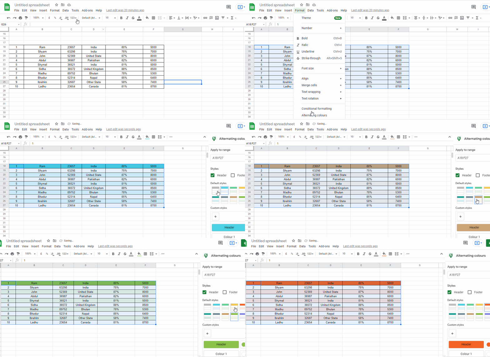
If you want to set a custom table color or automatic table color options then Google Sheets offers alternating color options in the table where you can automatically set the table color with just one single click and the whole table will be formatted with the color. You can also create custom color options to set table colors.
How To Make A Table In Google Sheets With Color Indicators
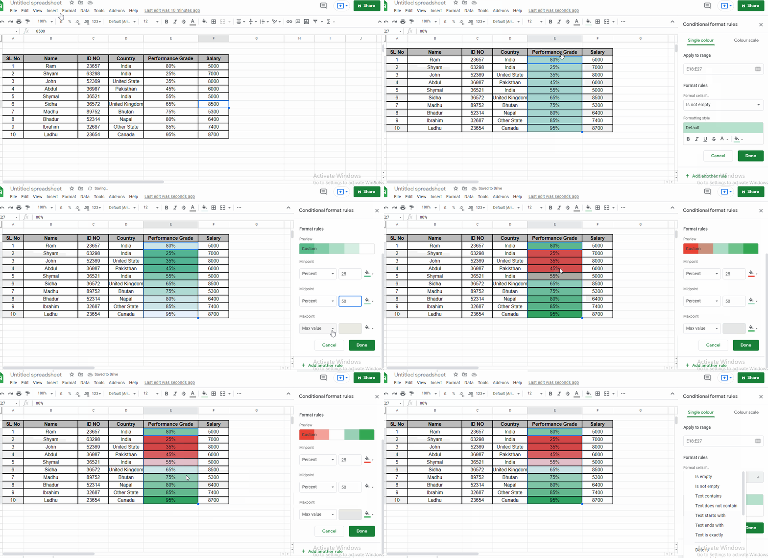
Google Sheets offers color indicators for your table row or column to draw more attention to that particular row or column. You can easily set the color indicators from the conditional formatting options and set the particular color or arrow or any other sign for the indicator options.
To set color indicators or any sign into your table first select the whole row or column on the table after that go to the format options after that you can find the conditional format options just click on the conditional format options and set the color or create any other rule for your column.
How To Add Link In Table
You can easily add any number of hyperlinks if you want that offer by Google Sheets. To add the hyperlink just select the text or number or anything that you write in the box and after selecting the particular field just click on the link options.
the link options you may find on the top right and after a click on the link just enter your link in the open box and hit the ok button. That's it.
The Final Word
In the above article, I will show you how to make a table in Google Sheets and format the table shows that the table looks very attractive. I will explain all the basic things on how to make a table in Google Sheets and make it beautiful but there are lots of things also available in Google Sheets the above table idea is very very basic for those who don't know anything about Google Sheets.
I hope you enjoy the article and if you think any basic things should be covered in the article then please write them down in the comment box below.


